3. Omics Data Analysis in Aging: Methylomics

Contents

• Omics Data Analysis in Aging: Methylomics

  • What is DNA methylation?

  • Why DNA methylation?

  • How to measure DNA methylation

  • How to analyze DNA methylation

    • Data processing and quality control

      • Processing bisulfite sequencing data

      • Processing microarray data

      • Looking at the data

    • Visualisation and statistical analysis

    • Interpretation and validation of DNAm analysis

  • Conclusions

  • Practice

  • Credits

  • References

3.1. What is DNA methylation?

Considering the previous chapters, you must have already seen that epigenetics plays a huge role in our lives. And indeed, epigenetic mechanisms tightly control all the intricate behaviors of our cells. Which functions to provide, which range of proteins to produce, and how to react to external signals: all of this information is not encoded explicitly in the DNA sequence, and is regulated by the epigenome [Lim et al., 2016]. There are a lot of various epigenetic mechanisms including histone modifications, nucleosome remodelling, noncoding RNAs, etc. [Saul and Kosinsky, 2021], however, DNA methylation is one of the most investigated types of epigenetic modifications. As you can see from the Fig. 3.1 below, we’re descending to the very depths of gene regulation.

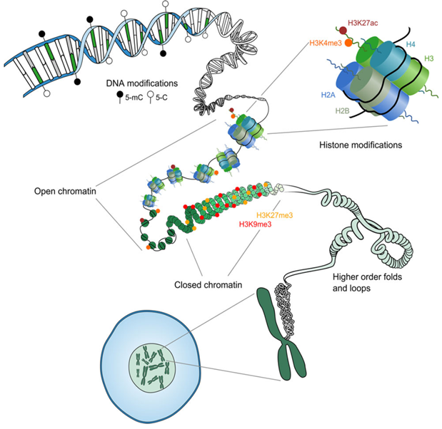
Fig. 3.1 Overview of epigenetic mechanisms [Hanna et al., 2018]

Methyl groups can be attached to the cytosine bases of DNA at the 5th carbon atom of the pyrimidine ring (annotated as 5mC), and it is most commonly observed in a CpG context (cytosine followed by a guanine nucleotide) [Seale et al., 2022], although other types of DNA methylation such as methylation of the nitrogen atom at the 6-th position of adenine (6mA) have also been discovered but remain poorly characterized [Iyer et al., 2016].

How does methylation appear? Well, there are two options (Fig. 3.2). First of all, DNA methyltransferase 3 (DNMT3) can produce methylation at the completely unmethylated sites (so-called de novo mechanism). Secondly, since CpG sites are symmetrical on both strands, it’s easy to imagine some mechanism that would recognise a site that is methylated at one strand and is unmethylated at the opposite one. Such situation occurs, for example, after DNA replication, where the mother strand retains its methylation pattern, but the daughter strand is built from raw nucleotides, so it’s not modified yet. In such cases, UHRF1 recognises these so-called hemi-methylated sites and recruits DNA methyltransferase 1 (DNMT1), which faithfully restores the symmetry [Greenberg and Bourc’his, 2019]. Both reactions require S-adenosyl methionine (SAM) as a donor of methyl groups.

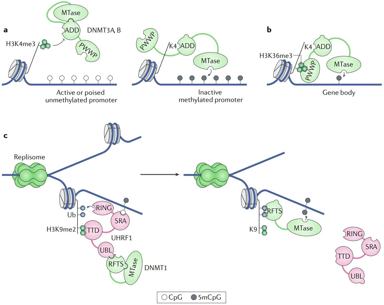
Fig. 3.2 Methylation pathways: de novo methylation by DNMT3A/B, a complex containing a conserved methyltransferase domain (MTase) and two histone reader domains, ATRX-DNMT3-DNMT3L (ADD) and PWPP, is (a) repelled by methylation at H3K4 and recruited by the binding of ADD to unmodified H3K4 in promoters and (b) enhanced by the interaction between PWWP and H3K36me3 in gene bodies; (c) maintenance methylation by DNMT1, a complex in which the catalytic MTase domain is blocked by its own replication foci targeting sequence (RFTS) domain, is mediated by the UHRF1 complex which recognizes hemi-methylated DNA using SRA domain, ubiquitinates H3 tails using RING domain, rescues DNMT1 from self-inhibition by binding to RFTS and targeting it to the ubiquitinated H3, thereby providing access of MTase to the unmethylated CpG site (adapted from [Greenberg and Bourc’his, 2019])

Demethylation is a less straightforward process. Up to date, no enzyme has been discovered that can directly convert methylated cytosines into unmethylated ones. Instead, ten-eleven translocation (TET) family enzymes can successively oxidize methyl cytosine to hydroxymethyl, to formyl, and to carboxyl cytosine, which is then excised from DNA by thymine DNA glycosylase (TDG). The empty space is recognised by the base excision repair system, which recruits a new cytosine to replace the excised one. In addition to this active pathway, methylation can be removed passively as a result of dilution during DNA replication [Greenberg and Bourc’his, 2019]. For example, if we imagine a case, in which, at the same time, cells divide rapidly, they replicate their DNA rapidly, and the UHRF1 or DNMT1 proteins are somehow inhibited, then there will be more and more cells with almost no methylation on both strands. This is what happens, for example, at the early stages of embryonic development.

DNAm is evolutionarily more ancient than the first eukaryote, nevertheless, it has been lost during evolution multiple times independently, likely because this modification is in fact quite toxic, since it can easily lead to spontaneous oxidative deamination of 5 methylcytosine into thymine [Iyer et al., 2016]. This is also the reason why the number of CpG sites in mammals, for example, is 5 times lower than expected from their nucleotide distribution. To make it even worse, DNA methyltransferase enzymes (DNMTs) are prone to produce 3mC instead of 5mC, thereby creating DNA lesions, and only co-evolution of methyltransferases with alkylation repair enzymes apparently allowed DNA methylation to be retained at all [Greenberg and Bourc’his, 2019].

It is important to note that due to a multitude of pathways and regulators, these processes of methylation (Fig. 3.2) and demethylation (Fig. 3.3) are in dynamic equilibrium to each other, and the exact point of balance is established for each CpG site at each cellular state.

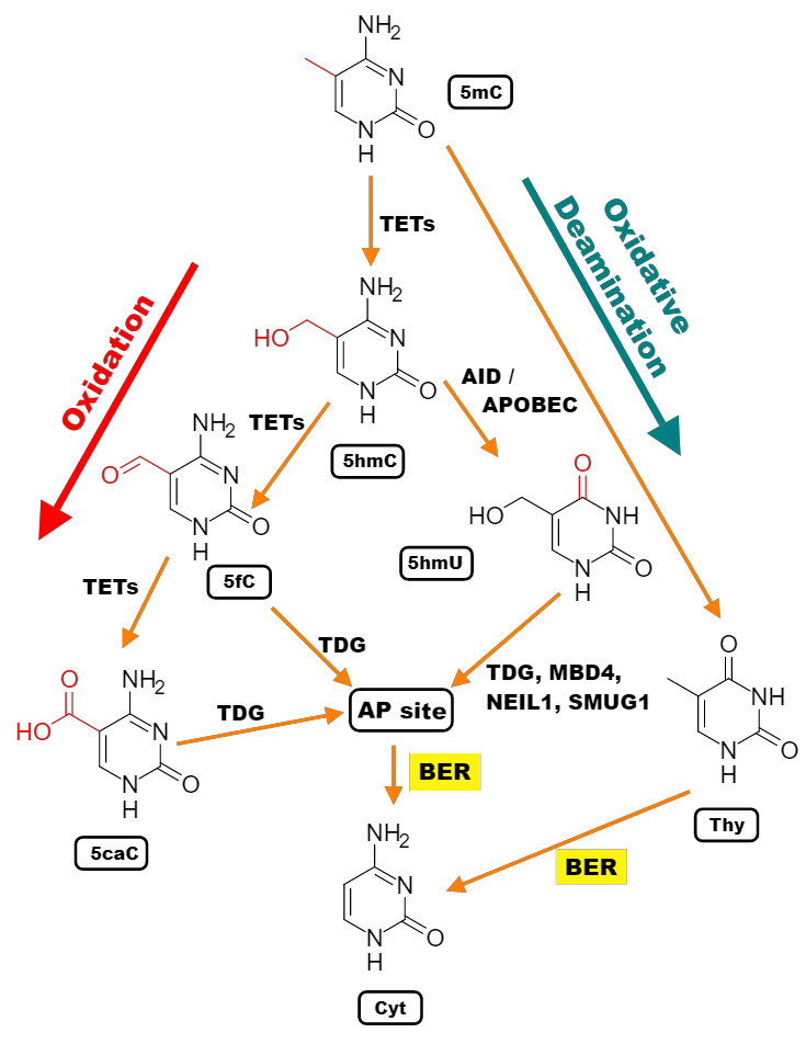
Fig. 3.3 Demethylation pathways: 5mC can be actively oxidized in a series of reactions mediated by the Ten-eleven-translocase (TET) family proteins to 5-hydroxymethyl- (5hmC), 5-formyl- (5fC), and 5-carboxycytosine (5caC) (noteworthy, each further step of oxidation occurs at a progressively slower rate [Ito et al., 2011]), whereupon 5hmC is converted to 5-hydroxymethyl uracil (5hmU) by the APOBEC (apolipoprotein B mRNA editing enzyme, catalytic) family members. 5fC, 5caC, and 5hmU can be excised, primarily by TDG, to yield an apurinic / apyrimidinic site (AP site) which is rescued by the base excision repair (BER) machinery. Alternatively, 5mC can spontaneously convert to thymine via hydrolytic deamination and then be subjected to BER as well [Bayraktar and Kreutz, 2018].

3.2. Why DNA methylation?

Now that we know, what DNA methylation is, it’s about time to find out what it does.

At some point, the “histone code” hypothesis was introduced in attempt to describe a certain pattern that governs which modification of which histone at which position serves a repressive or an activating function [Jenuwein and Allis, 2001]. However tempting it could be to assign these labels, considering the vast complexity of histone modification combinations, such a code might prove difficult to establish. Albeit, some patterns have earned enough credibility to be called “canonical” (Fig. 3.4).

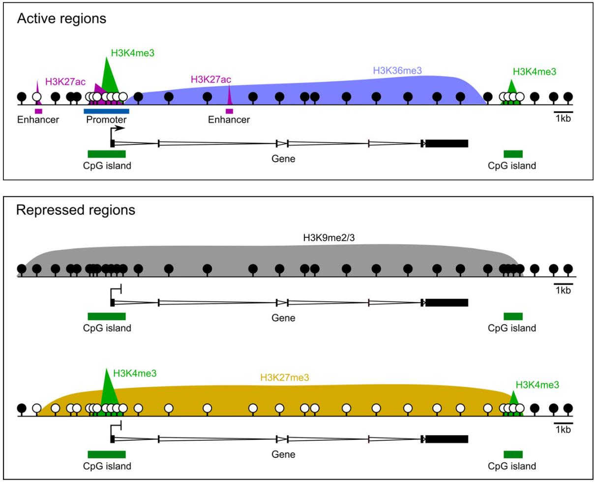
Fig. 3.4 Canonical epigenetic patterns. H3K4me3 is associated with active promoters and with CpG islands, regions of high genomic CpG occurrence, in general. H3K27ac appears at transcription-promoting regions (both promoters and enhancers), whereas H3K36me3 occupies transcribed gene bodies (supposedly, for prevention of spurious transcription and facilitation of already bound RNA polymerase). DNAm is usually highly methylated in gene bodies and intergenic regions, but is free of methylation at activating histones. On the other hand, transcriptionally inactive regions are usually fully covered with H3K9me2/3 or with H3K27me3 which overrides other activating histones and unmethylated DNA [Hanna et al., 2018].

As we can see from Fig. 3.4, DNAm is canonically repressive when occurs at promoter/enhancer regions. The reasoning behind is that methylated cytosine prevents transcription factors from binding to DNA, although even unmethylated cytosines can also be inaccessible upon H3K27 trimethylation. However, there are transcription factors with higher affinity to methylated cytosines in their respective binding motifs; for example, cell pluripotency factors KLF4 and OCT4, the homeobox proteins HOXB13, the NKX neural patterning factors, and C/EBPα [Greenberg and Bourc’his, 2019], which appear in the “Reprogramming” section of this paper.

In addition, methylation at regions upstream of promoters can evict Polycomb repressor complex 2 (PRC2) from there, thus preventing H3K27 methylation and activating transcription of these promoters, such as in the case of neural genes during neurogenesis, FOXA2 during endoderm development, and ZDBF2 in early embryos [Greenberg and Bourc’his, 2019]. In general, however, the main evolutionary role of DNAm is considered to be the support of genomic stability through silencing transposable genetic elements, which account for roughly half of human genomic space [Sanchez-Delgado et al., 2016], and other repetitive regions. This silencing is performed not only by TF inaccessibility, but also due to high rates of spontaneous and mutagenic deamination occurring in CpG-rich promoters of transposable elements [Greenberg and Bourc’his, 2019].

— Work in progress —

3.3. How to measure DNA methylation

The history of measuring DNA methylation is quite long (Fig. 3.5), and we’re not going to stop at every point of this timeline (if you’re eager to get the historical perspective, see [Li and Tollefsbol, 2021]), because most of these methods have long sunk into history. For example, even though liquid chromatography and mass spectrometry (LC-MS) is perfectly capable of profiling both 5mC, 5hmC, and all other DNA modifications, is never used for this task today because of its exorbitant costs.

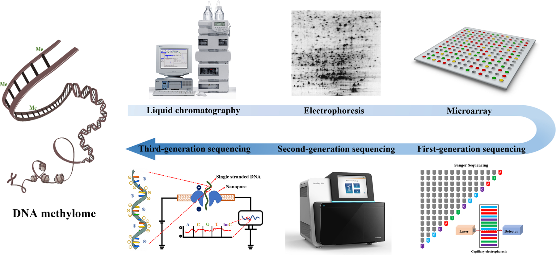
Fig. 3.5 Evolution of the DNA methylation profiling methods [Li and Tollefsbol, 2021]

Electrophoresis and first-generation (Sanger) sequencing methods are plainly outdated, while third-generation sequencing (Oxford Nanopore, PacBio) is too young and underdeveloped yet to be widely accepted by the epigenetics community. Only two methods survived the sands of time: microarray hybridization and second-generation sequencing, both of which we will discuss in more details today.

Essentially, the main take-home message from this chapter is that the microarrays represent an old technique that is relatively inaccurate, covers a small percentage of CpG sites, and is difficult to compare between different datasets (huge batch effect). However, it is still being upgraded (more CpGs are being included) and widely used, especially in human methylation profiling, for the only reason of its cost and ease of handling. Nevertheless, it is inevitable that the highly accurate and comprehensive (up to 100% of CpGs can be covered) sequencing-based methods, which have already become the “gold standard” in the field, will gradually replace microarrays as long as they become more and more affordable for the wider community.

Both microarray and sequencing technologies rely on amplification, during which DNA is fragmented, and the fragments are multiplied several times to increase their concentration. Across these steps, DNA methylation cannot be maintained, therefore, DNA should undergo some pretreatment which later allows distinguishing methylated from unmethylated. The main pretreatment methods are based either on [Li and Tollefsbol, 2021, Rauluseviciute et al., 2019]:

1. restriction enzymes (MRE-seq; Fig. 3.6, left column),

2. affinity enrichment (MeDIP-seq and MBD-seq; Fig. 3.6, center and right columns), or

3. bisulfite conversion (BS-seq, Fig. 3.7).

In MRE-seq, various methylation-sensitive restriction enzymes are used to cleave DNA at unmethylated sites, so DNA region methylation status can be deduced from the number of times a cutting site is observed (the more observations, the more methylated it is). The coverage of CpGs is therefore fully dependent on the range of cleavage sites that can be recognized by the enzymes. In MeDIP-seq, antibodies affine to 5-methylcytosines (or 5-hydroxymethylcytosines) are used to pull (“immunoprecipitate”) only methylated and single-stranded fragments from the solution. The main drawback of this approach is that the antibodies are biased to bind CG-rich fragments, yielding a lot of false negatives in CG-poor regions. In MBD-seq, methyl-CpG-binding domain proteins attach to the double-stranded methylated DNA fragments. Although, they cannot distinguish between 5mC and 5hmC, and bind unstably to the hemi-methylated DNA, yielding false negatives again. Most unfortunately, all affinity-based approaches are unable to profile methylation at single-base resolution, because whole fragments are pulled if they contain methylated CpGs, even though the unmethylated ones are also present.

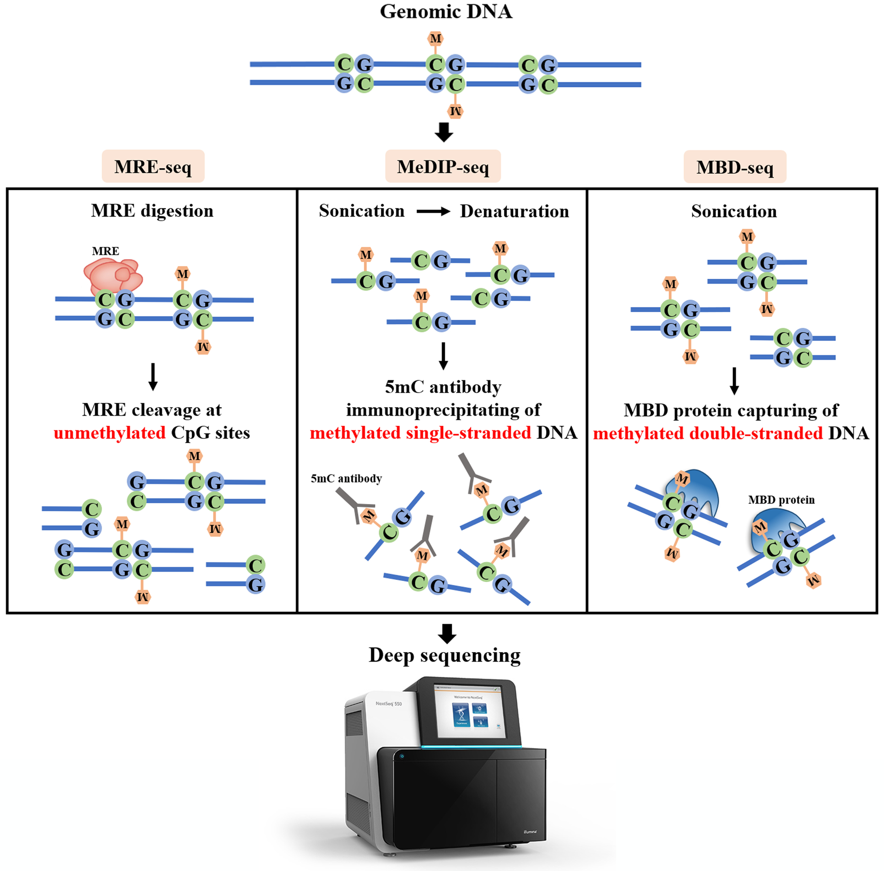
Fig. 3.6 Restriction enzymes-based and affinity enrichment-based methods for DNA methylation profiling [Li and Tollefsbol, 2021]

Bisulfite conversion is the most widely adopted approach for DNA methylation profiling. In it, DNA is treated with sodium bisulfite, which converts unmethylated cytosines into uracils (replaced with thymine during amplification), while methylation provides protection from this conversion, so 5mC remains intact. As a result, 5mC will be read as C, while unmethylated C becomes T. Comparing the converted fragments with the reference genome allows resolving modified cytosines from the unmodified ones. The main sources of bias in BS-seq are incomplete BS conversion, BS-induced DNA degradation, PCR amplification, and DNA modifications (both 5mC and 5hmC are protected from BS) [Li and Tollefsbol, 2021]. Still, it provides the greatest accuracy, reproducibility, and coverage, so our further discussions will only be related to the post-BS conversion approaches.

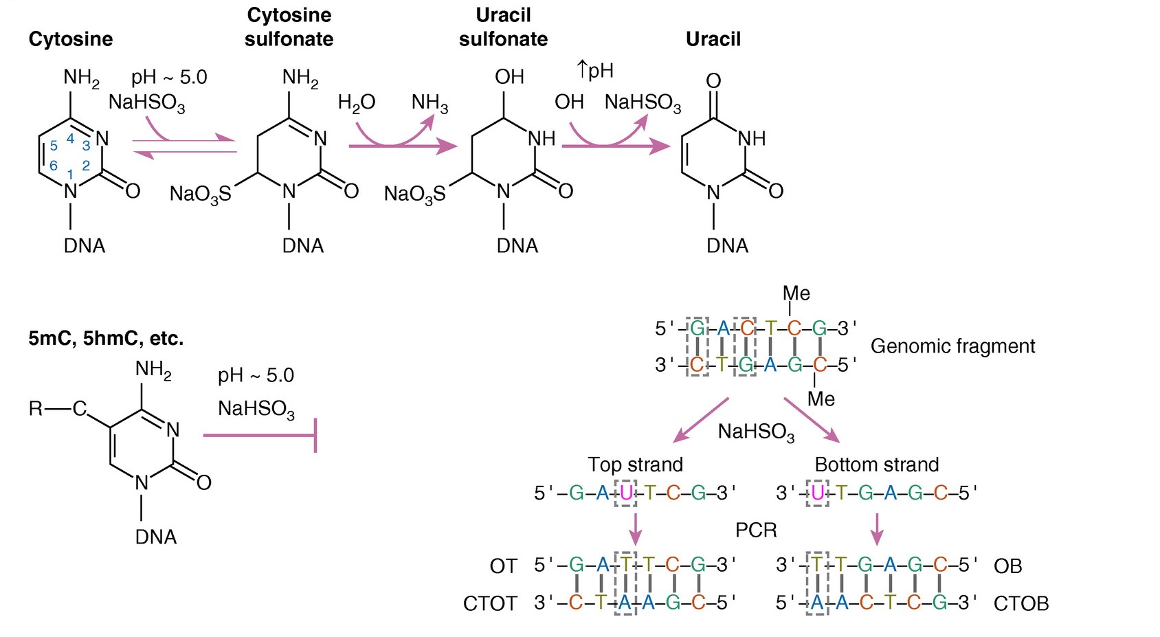
Fig. 3.7 Schematic representation of the bisulfite conversion reactions and resulting DNA fragments, adapted from [Singer, 2019]

Finally, after pre-treatment is done, DNA fragments are sent either to bead chip microarrays or to deep sequencing machines. In microarrays, essentially, DNA fragments bind to the arrays of short nucleotide beads attached to a chip. The binding is based on whether these fragments are complementary to the bead sequences. Therefore, DNAm coverage fully depends on whether a particular sequence is present in the beads. The DNAm BeadChip microarray technology is advanced by the Illumina company and has been through four generations with successive increases in methylome coverage: ~1.500 CpGs (in promoters), ~27k CpGs (in promoters), ~450k CpGs (in promoters and proximal enhancers), and ~850k CpGs (adding sites in distal enhancers to the 450k coverage). Both 450k and 850k platforms are still widely used, especially in the human cancer studies.

Sequencing is done either across the whole genome (whole genome BS, WGBS) or after the isolation of CpG-rich regions by applying restriction enzymes prior to bisulfite conversion (reduced representation BS, RRBS). RRBS was developed as a compromise between covering a large proportion of methylome, while discarding methylation sites far outside of CpG islands, thus substantially reducing the sequencing costs (although some CpG-rich regions remain uncovered due to the restriction enzyme specificity) [Li and Tollefsbol, 2021].

Some of the aforementioned methods have been adapted to profile 5hmC and other DNA modifications in addition to or instead of 5mC. In terms of profiling methylation in single cells, numerous approaches (BS-based, primarily) have been suggested that often combine it with the profiling of transcriptomics, chromatin openness, histone modifications, etc. [Ahn et al., 2021]

Combinatorial strategies have been gaining attention in the past decade, for they allow profiling DNA methylation simultaneously with other epigenomics or transcriptomics features. For example, in NOMe-seq, the addition of GpC methyltransferase before bisulfite sequencing provides both DNA methylation and nucleosome occupancy (i.e., accessibility of DNA regions for transcription) profiles. NOMe-seq and other techniques, sometimes coupled with capturing single cells (sc), such as ChIP-BS-seq (DNAm + histone modifications), scCOOL-seq (DNAm + chromatin accessibility) scNMT-seq (DNAm + chromatin accessibility + transcriptomics), etc. [Ahn et al., 2021, Minnoye et al., 2021] are paving the road for comprehensive understanding of biological processes on a whole new multi-omics level.

In the end, the choice of DNAm profiling methods stems from the cost-effectiveness considerations and posed biological questions. While it is undoubtedly beneficial to comprehensively profile whole methylomes at single-base resolution using WGBS, the costs of such an endeavor make researchers resort to the less comprehensive and more biased, although far more affordable approaches such as RRBS and microarray technologies. The features, advantages, and disadvantages of the methods we’ve discussed here are displayed in Table 3.1 (adapted from [Li and Tollefsbol, 2021, Rauluseviciute et al., 2019, Singer, 2019]).

Table 3.1 DNAm profiling methods overview (assembled from the papers mentioned previously in this section)

Profiling Method	Pre-treatment	Target	Context	5mC / 5hmC	Coverage	Quantification	Wet lab requirements	Sources of bias	Costs
MRE-seq	Restriction enzymes	Cleaves at unmethylated	CpG	5mC only	Low (<6% of CpGs, depends on restriction sites)	Relative	Low	Restriction sites, fragment size	Low
MeDIP-seq, MBD-seq, etc.	Affinity enrichment	Pulls at methylated	CpG	Either	Medium (60-85% of CpGs)	Relative	Low	Copy number, CG content, CpG density	Low to medium
Microarray-based	Bisulfite conversion	Converts C, intact 5mC	CpG (specified by probe sequences)	Merged	Low (specific sites, <5% of CpGs)	Absolute	Medium (specialized platform)	Background correction, inter-array normalization, probe-design bias, dye bias	Medium
WGBS	Bisulfite conversion	Converts C, intact 5mC	Any	Merged	Highest (up to 100% of methylome)	Absolute	High (specialized chemistry and computational platforms)	Incomplete conversion, PCR artifacts	Very high
RRBS	Bisulfite conversion	Same as WGBS, but at CG-enriched	Any (mostly CpG)	Merged	High at CGIs (85%), low in total (13% of CpGs)	Absolute	High	Incomplete conversion, PCR artifacts	High
oxBS-seq	Bisulfite conversion	5hmC	Any	Both	High	Absolute	High	Incomplete conversion, PCR artifacts	Very high
TAB-seq	Bisulfite conversion	5mC	Any	5hmC only	High	Absolute	High	Incomplete conversion, PCR artifacts	Very high

3.4. How to analyze DNA methylation

Computational analysis of DNA methylation consists of three main steps [Bock, 2012, Rauluseviciute et al., 2019]:

1. Data processing and quality control

2. Visualization and statistical analysis

3. Validation and interpretation

We will briefly outline this workflow and discuss some important caveats that arise during each step. Bisulfite conversion-based approaches are of the most interest to the researchers nowadays, so we will omit the peculiarities of other approaches to DNAm profiling here (if you’re that interested, see [Bock, 2012, Rauluseviciute et al., 2019]).

3.4.1. Data processing and quality control

3.4.1.1. Processing bisulfite sequencing data

Processing raw bisulfite sequencing data must deal with the following tasks:

1. Trim sequencing adaptors from the ends of reads (adaptors are added to reads to improve capturing of the smaller-sized ones) and trim reads with low quality (e.g., incorrectly converted)

2. Align (or map) reads to the reference genome

3. Calculate methylation fractions (or beta values) per site

Trimming is, to some extent, a trivial task, and tools for trimming have been largely adopted from other omics data analyses such as DNA-seq or RNA-seq.

Read alignment, however, is rather challenging, because bisulfite conversion produces reads with reduced complexity (far fewer cytosines than in the original sequence), which increases chances to observe a read that can be mapped to multiple genomic regions. But more importantly, alignment algorithms must take into account that some of the Ts it observes in the reads are originally Cs (in the reference genome). To overcome this problem, two main branches have been proposed: wild-card aligners and three-letter aligners.

Wild-card aligners (such as BSMAP) substitute every C in the reference by the wild card Y, which can be aligned to both C and T in the sequencing reads. As can be seen from an example in Fig. 3.8, wild-card aligners may introduce bias by overestimating methylation proportions (methylated reads contain Cs that raise read sequence complexity enough so that these reads can be mapped unambiguously, but the unmethylated reads bearing Ts are prone to be discarded because they align to different genomic regions simultaneously).

On the other hand, three-letter aligners (such as Bismark or BS Seeker) that replace every C in the reference genome with a T (therefore, only three letters from the genomic alphabet are left: A, G, and T) are simpler in use (because conventional genomic aligners can be employed) and are not biased towards overestimating or underestimating methylation fractions. However, since they reduce sequence complexity even more, a large fraction of reads aligns ambiguously and is discarded (Fig. 3.8).

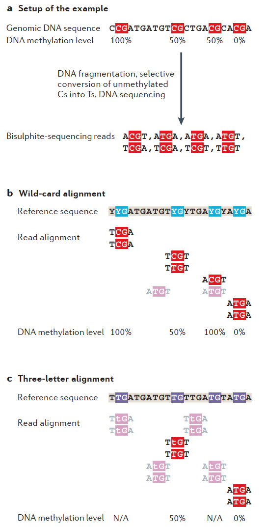
Fig. 3.8 Strategies for bisulfite alignment [Bock, 2012]

In conclusion, wild-card aligners provide higher coverage at the cost of overestimating methylation, while three-letter aligners yield precise values, but only for a fraction of reads, at the expense of losing coverage. It is worth noting that profiling genomic regions with higher sequence identity (containing transposable elements or duplications) or using shorter reads suffers the most from the aforementioned issues [Bock, 2012]. As a result, even though WGBS theoretically covers up to 100% of a methylome, it cannot be achieved in practice due to the methodology of three-letter alignment, although newer algorithms are doing their best to increase their output coverage [de Sena Brandine and Smith, 2021, Huang et al., 2018].

After performing the alignment, we can calculate methylation fractions by simply dividing the number of observed Cs by the sum of Cs and Ts per methylation site, and it is exactly what most researchers do. However, additional post-alignment adjustments can improve the accuracy of this approach: for example, it does not distinguish between the bisulfite conversion-induced Ts and genetic variants. The Bis-SNP variant caller (an extension of a popular Genome Analysis Toolkit, GATK) attempts to deal with this bias by leveraging the fact that “bisulphite‑induced C‑to‑T variants exhibit a G on the opposing strand, whereas genetic C‑to‑T variants exhibit an A instead” [Bock, 2012], along with being handy in the SNP analysis in general [Liu et al., 2012]. In addition to all that, the success rate of bisulfite conversion is another metric that should be accounted for. Quality control of this rate can be performed by adding standardized DNA with known DNAm values, either pre-constructed oligomers or methylation-free viral DNA.

As you can see, there are enough steps to be worried about if you want to process your data in the best way possible. Although multiple comparison reviews are out there, almost none of them attempts to provide actual guidelines on which tools would be better to use in which circumstances, and, since the techniques are updated and developed every year, even those reviews that do try to suggest such ‘gold standards’ [Rauluseviciute et al., 2019] are quite outdated, so the researchers have to choose on their own.

3.4.1.2. Processing microarray data

The Illumina microarrays are, on the one hand, easier to process than sequencing results (no alignment required, since probes contain pre-defined sequences), but, on the other hand, are far more laborious.

Instead of sequencing reads, microarrays provide colour signals of different intensities across a time range. The coloured image processing is virtually always done with the vendor-supplied software, so you won’t have to bother about it. However, after the signals are counted, the bioinformatician’s work begins.

First of all, just as with bulk BS-seq, bias may arise from sample DNA composition (polymorphisms or cell heterogeneity), but, more importantly for the microarray methodology, bias comes from the arrays themselves:

• cross-reactions between probes,

• background bias,

• nonlinear dye bias,

• probe-type bias (starting from Infinium 450k, probes are manufactured in two types, each with its specific characteristics, and both are present in every platform),

• and batch effects between two arrays.

We are not trying to become full-stack DNA methylation bioinformaticians in the scope of this course, so we will not go into full discussion about all these and about a whole battery of various normalization and bias correction approaches that have been described specifically to tackle these problems with microarray data (if you do want to delve deeper, see reviews [Nakabayashi, 2017, Welsh et al., 2023, Wu et al., 2014]). In short, SeSAMe coupled with pOOBAH filtering (SeSAMe 2) appears the best performing microarray processing algorithm [Welsh et al., 2023], although it is a relatively young tool, so you will rarely encounter datasets processed by it. More often, researchers resort to the good old practices such as the default pre-processing steps of the minfi R package (quantile normalization for blood and DLPFC samples and noob procedure otherwise, according to the minfi manual).

In the end, even if you use only the best processing tools, microarrays are still notorious for their between-array batch effect. Wet lab researchers are highly advised to profile samples in mixed order so as to minimize the magnitude of potential confounders (for example, to process samples from different tissues or the case and control samples on the same day, and not on different weeks). However, you will unlikely get this information from the open-source databases, and you will certainly be unable to change the way the datasets are collected. Several batch correction techniques are implemented in the aforementioned approaches, and there are also specific tools (e.g., ComBat, surrogate variable analysis (SVA), RUVm, etc. [Nakabayashi, 2017]), but they still have quite a room for improvement [Ross et al., 2022, Zindler et al., 2020].

3.4.1.3. Looking at the data

Further in our course (and in a lot of research settings, really), you will be spared from processing the raw reads, so let’s briefly overview how the actual processed DNA methylation matrix looks like.

For bisulfite sequencing, it comes in a variety of data formats. The major separation lies between the binary files (e.g., .bigWig) and the more familiar tab/comma-separated text files (e.g., Bismark .cov files, BS-Seeker .CGmap files, .bed and .bedGraph files, etc.). A lot of processing tools employ their own data format, so the format you get to work with depends on what you (or the authors of your dataset) have chosen to process your reads.

The main information that is always present in these files is genomic position (chromosome and DNA base number) and methylation level (a.k.a. methylation fraction or beta value). Ideally, to perform quality control on your sites, you want to also know the coverage—total number of counts (methylated + unmethylated)—per site, which is not always readily available (in case of .bigWig, for example). As DNAm may occur on both strands, but the annotation is done against the positive (Watson) strand positions only, some formats also mention the strand directionality per DNAm site (+/- or F/R), but some do not, so you might want to look at the reference genome to infer this information. Other columns may include the information on methylated and unmethylated counts, on the genomic context around a DNAm site (CpG, CHG, CHH, where H stands for ‘not G’), or something else. A good example of how processed DNAm data looks like is displayed in the BS-Seeker3 manual (Fig. 3.9), although most of these columns are usually absent in the outputs of common processing frameworks (e.g., Bismark .cov).

The other caveat you should be aware of is genomic positioning. As you can see from Fig. 3.9, BS-Seeker uses single-base notation (column 3), but it’s not always the case. Some pipelines output two-base notation, some even employ three-base regions, but you should not be misled: all of these regions involve only one DNA methylation site. In the 1-base case, it’s obvious to see where exactly it lands; in 3-base, it’s usually the position in-between the starting and ending positions; but the 2-base case is probably the most misleading, as it can be both. We advise you to always check your notation against the reference genome (UCSC browser will suffice) bearing in mind strand directionality, if you’re dealing with more than one dataset (especially if they’re processed by different tools), which often happens when building and using methylation clocks, for example.

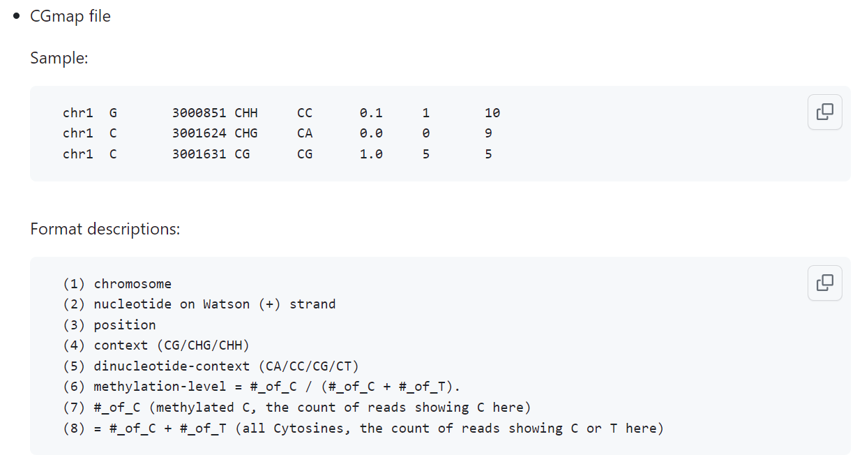
Fig. 3.9 Example of processed DNA methylation data (BS-Seeker3 CGmap formatting)

Files after microarray processing are similar, but a ton more uniform:

• they are mostly tab/comma-separated text files,

• genomic positions are always notated in the Illumina ID style (this is an important caveat, since you have to convert these IDs into common genomic coordinates if you wish to compare microarray and BS-seq datasets, e.g., Illumina cg07881041 corresponds to chr19:5236005 in the hg38 human genome assembly),

• no strand information (can be inferred from genomic positions),

• context is always CpG,

• no counts (instead, there are methylated and unmethylated signal intensities, which are to be discarded after calculating methylation fraction values).

To sum up, the only info you can get directly from the processed microarray data is CpG site ID and its methylation level. Extremely user-friendly. Especially if you forget about all the numerous normalizations and bias corrections that have led you to these methylation levels.

3.4.2. Visualisation and statistical analysis

Finally, after methylation percentages are calculated, we step into the realm of data analysis and interpretation. The amount of tools and approaches available for it is overwhelming, so we will only mention a few.

One of the obvious direct approaches is to look at your data, which can be done via the good old UCSC Genome Browser, SeqMonk, the Integrative Genomics Viewer (IGV), or many other tools [Bock, 2012]. In addition to visualizing methylation profiles, it is also useful to perform some form of unsupervised dimensionality reduction, for example, by principal component analysis (PCA) or hierarchical clustering, to elucidate the major groups of samples in your data (and to detect some outliers).

But of course, probably the most widely adopted approach is to find differentially methylated (DM) positions (a.k.a. DMPs, DMSs [sites], or DMCs [CpG sites]) or regions (DMRs) by comparing two or more studied groups, for example, to find differences between DNA methylation in a certain cancer type and healthy controls, or between cancer types. And, essentially, the main goal of DNAm profiling in the first place is to identify systematic differences between samples and sample groups, which is exactly the job for DM analysis.

DMP analysis is more suitable for the microarray-based data, since a lot of genes there are covered with only one CpG site, or several sites are spread too far apart from each other (e.g., one is situated in a promoter, and another one is in a gene body). In WBGS and RRBS, on the other hand, a promoter can be covered with a dozen of CpG sites, and the variation at each of them can be a lot higher than the variation of methylation across the whole promoter (due to sequencing variability). In addition to that, DNAm sites are known to correlate really well within CpG islands, or in otherwise close proximity to each other [Affinito et al., 2020]. Therefore, it is logical to interrogate DNA methylation not at individual sites, but in whole regions, which can be derived by splitting genome either into equally sized ranges, or into CpG-dense fragments (especially relevant for RRBS) [Chatterjee et al., 2017]. There are numerous statistical approaches to calculating differential methylation, whose pros and cons have been thoroughly discussed and reviewed elsewhere [Piao et al., 2021, Shafi et al., 2018]. The key feature in these approaches is the statistical test they use to estimate statistically significant differences in DNAm levels. Model assumptions about how DNAm levels per site/region are distributed and different genome segmentation methods are also embedded into these approaches, so the outcomes of their work (i.e., discovered DMRs) are inevitably different.

Another, less widely adopted, but still pretty insightful method is the analysis of methylation variability (again, at individual positions, VMPs, or at regions, VMRs), since variable methylation has also been linked to cancers, diseases, and aging [Seale et al., 2022]. For example, increasing variance of housekeeping genes was shown to predict chronological age and aging-associated pathologies with even greater accuracy than methylation clocks built on changes in mean DNAm [Mei et al., 2023]. Approaches to VM analysis are numerous as well, and are compared elsewhere [Li et al., 2015].

It is worth to keep in mind that methylation differences and variations may actually arise not from changes in DNAm profiles themselves, but from changes in cell composition: for instance, it is well-known that, during aging, the distribution of immune cells in blood shifts strongly towards the myeloid lineage cells [Nishi 2019], which likely affects training epigenetic clocks on bulk blood DNAm data. Therefore, it can be useful to assess cell-type heterogeneity between sample groups, which has also been reviewed in great length elsewhere [Teschendorff and Relton, 2018].

All things combined, evaluating differences in mean DNAm, in DNAm variance, and in DNAm heterogeneity (Fig. 3.10) provides a multi-dimensional outlook on epigenetic alterations, which may help us elucidate disease- and age-related features of the epigenome.

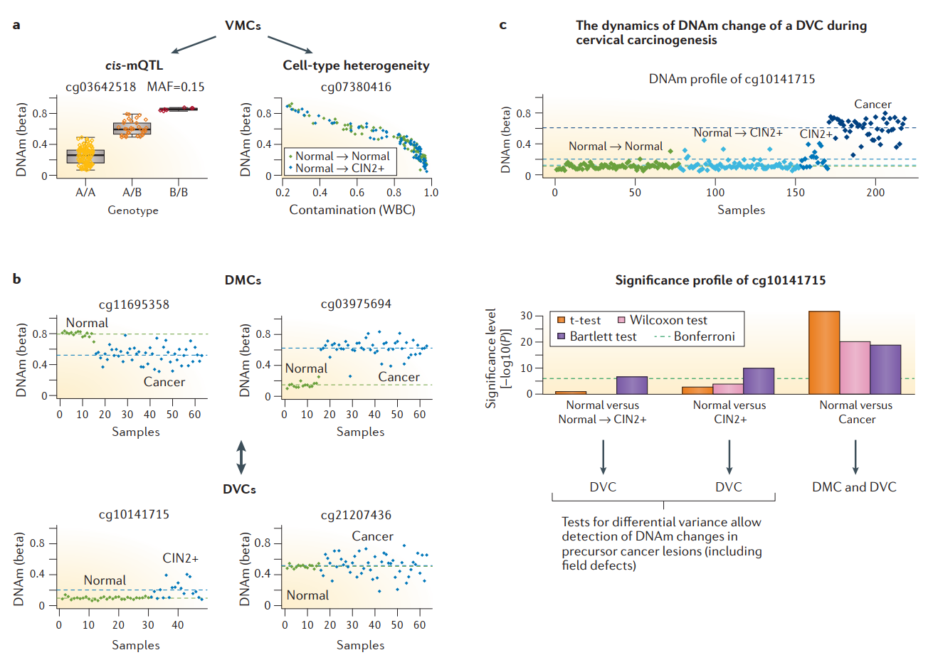
Fig. 3.10 Combining differential DNAm, variable DNAm, and cell-type heterogeneity in DNAm to compare healthy epigenome with progressing cancer epigenetic profiles: (a) two examples of VMCs, one driven by single-nucleotide polymorphisms (SNPs) located in cis with the indicated CpG site (defining a well-known cis methylation quantitative trait locus (cis-mQTL)) (left panel) and another driven by variation in immune-cell contamination (right panel). Panels illustrate how SNPs and cell-type composition can drive large variation in DNAm, while variation may not correlate with case versus control status. (b) Contrast between DMCs and DVCs. drawn from normal cervical smears (green) and either cervical intraepithelial neoplasia (CIN2+) or cervical cancer (both blue). Observe how a DMC is typically characterized by most samples in one phenotype exhibiting a deviation in DNAm value. By contrast, a DVC is characterized by a very stable DNAm profile in one phenotype but by DNAm outliers driving large variation in the other. (c) Example of a CpG that exhibits progression in DNAm between successive stages in cervical carcinogenesis. When comparing normal cervical smears that progress to CIN2+ to those that do not (Normal → Normal), this CpG can be identified only via a test for differential variance. When comparing CIN2+ to normal cervical smears, differential variance is still the main distinguishing feature. Only when comparing (invasive) cervical cancer to normal cervix does this CpG exhibit a stronger difference in average DNAm. Thus, this panel emphasizes the importance of selecting the appropriate statistical test, as the choice of test will have a dramatic impact on feature selection. (Adopted from [Teschendorff and Relton, 2018])

Another approach is to raise the stakes of dimensionality by investigating interconnected and co-methylated groups of DNAm sites or regions on the level of whole methylomes instead of looking for changes in individual sites or regions, since long-range genomic interactions are as prominent and influential as the short-ranged ones thanks to chromatin folding and compactization. Weighted gene co-expression network analysis (WGCNA) was initially developed to study such interconnected groups in the context of gene expression, but it was later leveraged for other omics data, including methylomics [Seale et al., 2022].

The core principle of WGCNA is to use network language to integrate individual nodes (genes or DNAm sites) of complex systems into clusters in an unsupervised manner and infer biological insights from how these clusters behave from sample to sample.

The main steps of WGCNA are to [Rezaie et al., 2023, Seale et al., 2022] (Fig. 3.11):

1. Measure pairwise correlations between nodes (genes or DNAm sites).

2. Calculate proximity between nodes based on these correlations.

3. Construct correlation network based on proximities by computing a topological overlap matrix (or TOM).

4. Find clusters (modules) of closely connected nodes via hierarchical clustering and dynamic tree cutting (to merge some of the least differing clusters).

5. Combine the information about all nodes per module in a sample using dimensionality reduction techniques such as SVD (singular value decomposition) and extract the first component of this “summary” (a.k.a., the eigengene)

6. For every node, calculate its correlation with the module’s eigengene, therefore inferring module membership for this node. Nodes with highest module membership are the ones that lie at the network’s core and are called “hub” nodes.

7. Correlate modules with experimental traits and compute eigengenes for every experimental sample category.

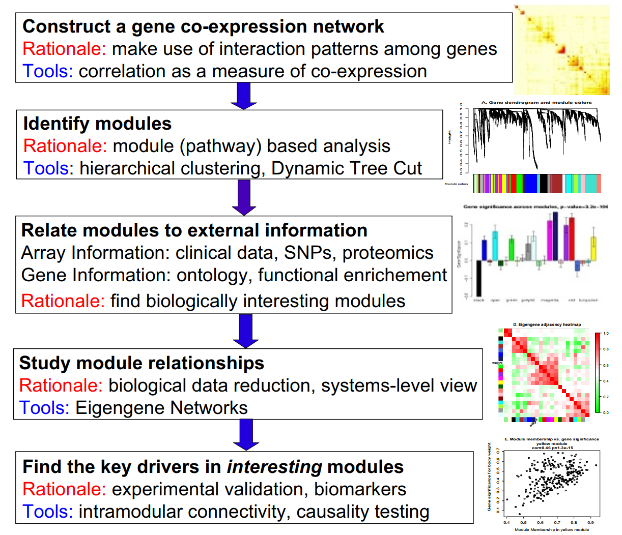
Fig. 3.11 WGCNA pipeline [[]]

Such systemic approach allows uncovering less obvious interactions and changes than the trivial comparisons of average or variable methylation levels can provide.

3.4.3. Interpretation and validation of DNAm analysis

Nevertheless, making biological assumptions or, even better, theories based on DNAm analysis is still enormously challenging.

The first step towards interpreting DNAm analysis is similar across many omics data analyses: functional enrichment, which is usually performed by identifying outstanding gene ontology (GO) terms, KEGG pathways, or REACTOME interactions for the DNAm sites, regions, or modules that were selected during the previously described analyses. It’s worth noting that, since covered DNAm sites may (and, in some methodologies, must) be distributed unequally across different genes, identified DMPs and VMPs should be adjusted so as not to over-represent some genes due to this technical variability alone. Alternatively, DNAm sites across certain regions can be combined: for example, assigned to gene promoters (if they fit within certain distance from the transcription start sites, TSS, of these genes) or enhancers, which are only then sent to the common gene set enrichment analysis (GSEA) tools [Teschendorff and Relton, 2018].

Not without certain difficulties, DNAm data can be integrated with genotyping data (approximately 20% of inter-individual DNAm variation is explained by genetic variation, so it should be adjusted for this inheritance, especially in the non-inbred study organisms such as outbred mice or humans), gene expression data (in general, DNAm is a bad predictor for expression levels, significantly worse than histone modifications are, but some parts of gene’s DNAm sites may be more predictive than others, although the exact correlations are still being debated, and more consistency is required), and with other omics modalities.

On the system level, comparing WGCNA-selected modules between sample groups or even datasets may shed light on how conserved these modules are: for example, a recent paper reported finding modules correlated with maximum lifespan by comparing DNAm profiles of a multitude of mammalian species (Fig. 3.12). In addition, the same paper also connected different modules to different behaviors in response to pro-longevity interventions such as growth hormone receptor knockout, caloric restriction, or cellular reprogramming mediated by applying four transcription factors (so-called Yamanaka factors) [Haghani et al., 2023].

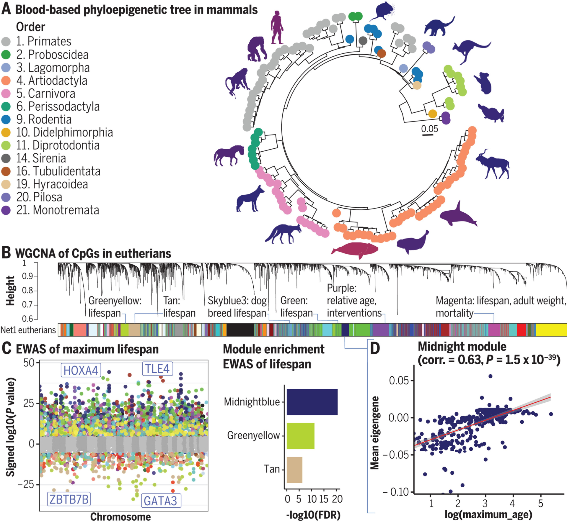
Fig. 3.12 DNAm network relates to mammalian phylogeny and traits. (A) Phyloepigenetic tree from the DNAm data generated from blood samples. (B) Unsupervised WGCNA networks identified 55 co-methylation modules. (C) EWAS of log-transformed maximum life span. Each dot corresponds to the methylation levels of a highly conserved CpG. Shown is the log (base 10)–transformed P value (y axis) versus the human genome coordinate Hg19 (x axis). (D) Co-methylation module correlated with maximum life span of mammals. Eigengene (first principal component of scaled CpGs in the midnightblue module) versus log (base e) transformed maximum life span. Each dot corresponds to a different species [Haghani et al., 2023].

Another system-level approach is to “integrate DNAm and gene expression data in the context of a gene function network, for instance a [protein-protein interaction] PPI network, to identify hot spots (gene modules) where there is significant epigenetic deregulation in relation to some phenotype of interest” [Teschendorff and Relton, 2018]. Such approach is called a functional epigenetic modules (FEM) algorithm, which, for example, “successfully identified two separate gene modules with the main targets of epigenetic silencing mapping to a target (HAND2) and co activator (TGFB1I1) of the progesterone receptor, a key tumour suppressor pathway for which inactivation is thought to contribute causally to the development of endometrial cancer” [Teschendorff and Relton, 2018].

The causality of DNAm dynamics is another great area of research, and is still largely underdeveloped. As you could notice, we’ve been mostly talking about correlations and associations for the past several paragraphs. But, as we all know, correlation does not imply causation. Especially since reverse causation (biological feature may influence DNAm at a particular site stronger than vice versa) Even more sophisticated frameworks are needed to resolve how methylation affects other layers of biological systems.

Of course, in some cases, researchers try to prove causality directly by editing some DNAm sites or by doing some other kinds of experimental validation, and these approaches will likely remain the “gold standard” of causality studies, but they all are painfully unscalable. Therefore, computational algorithms are being developed to yield some evidence on causality by other means, the most prominent examples of them being (Fig. 3.13):

1. Exposure-outcome mediation (EOM; the effect of exposure on an outcome is tested to be statistically significant once adjusted for DNAm-mediation): simple and quantifiable, but too assumptive and rigid (relies on complete, not partial mediation, which is not the case for DNAm).

2. Causal inference test (CIT; similar to EOM, but replaces exposure with genotype [mQTLs]): less prone to confounding and reverse causation, since it relies on genotype anchoring, but it fails to estimate the magnitude of the mediated effect, and doesn’t account for other possible mediation routes, along which genotype may affect outcome (pleiotropy).

3. Mendelian randomization (MR; in essence, it uses established relationships between genotypes [mQTLs] and exposures or mediators of interest to estimate the effects they have on some outcome, or vice versa; for deeper dive into theory behind MR, read [Davey 2014]): estimates effect magnitude, smaller measurement error, more robust against pleiotropy, but relies wholly on the availability of mQTL identification, and requires large sample sizes.

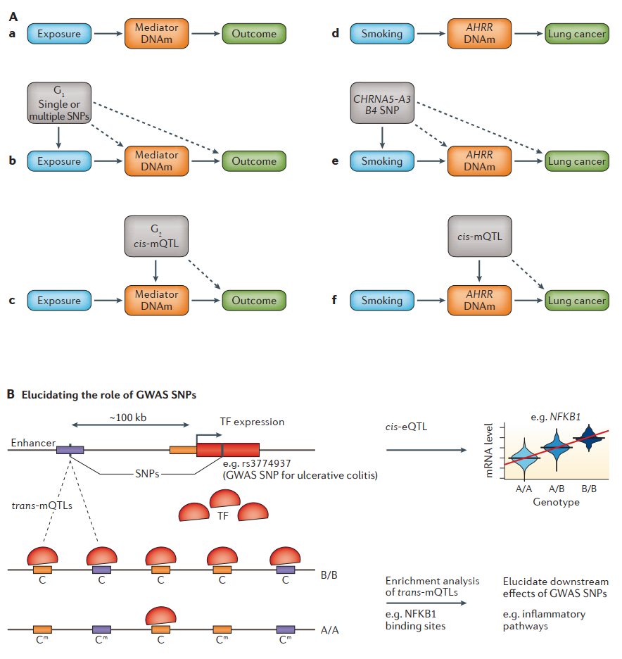
Fig. 3.13 Integrative approaches to the interpretation of DNA methylation data. (Aa) General causality framework exemplified by that (Ad) AHRR gene methylation is strongly associated with smoking and lung cancer risk. (Ab) To strengthen causal inference from exposure to outcome and from exposure to mediator, a genetic variant (G1) or combination of multiple variants that robustly correlate with the exposure can be used (such as (Ae) SNPs at the CHRNA gene that are established correlates of heavy smokers). Solid lines represent the established association of the instrumental variable (SNP) with the factor for which it is acting as a proxy, and dashed lines represent the relationships being tested in the Mendelian randomization (MR) framework. The association of G1 with the outcome (and mediator) provides evidence of a causal impact of the exposure on these factors. (Ac) When considering the causal pathway from the mediator (DNAm) to the outcome, a second genetic variant (G2) or combination of multiple variants can be used. G2 is a cis methylation quantitative trait locus (cis-mQTL) that robustly correlates with the DNAm site of interest. G1 and G2 analyses can, if desired, be conducted in entirely different sample sets with causal inference remaining valid. (B) Integration of DNAm data with matched SNPs and mRNA expression can be used to elucidate the role of genome-wide association study (GWAS) SNPs. For instance, a genetic variant defining a cis expression QTL (cis-eQTL) for a transcription factor (TF) can be found to be associated with a large number of trans-mQTLs. For cis-eQTLs associated with increased TF activity, these trans-mQTLs exhibit a skew towards hypomethylation (loss of methylation is indicated by the transition Cm (methylated cytosine) to C (cytosine)) and are enriched for binding sites of this TF and for cis expression quantitative trait methylation loci (cis-eQTMs) defined by the corresponding TF gene targets. An example of a SNP associated with ulcerative colitis illustrates how relevant disrupted pathways can be identified (adapted from [Teschendorff and Relton, 2018]).

In the end, we’d like to also mention that DNA methylation has been used quite extensively in a variety of ways to construct so-called epigenetic aging clocks and predict acceleration or deceleration of biological aging in various research environments. However tempting it would be to rush into this hyped up field, we shall restrain ourselves for now, since we’re going to have a full other chapter dedicated to aging clocks. Just don’t forget about our discussion on DNAm causality when you’ll be heading your way into it.

3.5. Conclusions

DNA methylation is a fascinating biological feature that interacts with so many other layers to regulate cellular functions. It finds its way in a lot of different disease states, heritable traits, early-life-induced repercussions for mental and general health, and into aging.

Nevertheless, measuring and analysing it is still substantially challenging, both in regards to computational resources and skills, and in terms of theoretical foundations for inferring causal interactions rather than just associations.

We are extremely delighted if you have managed to reach this point of our lengthy discussion, and if you find yourself in a more cognizant position than where you were when starting it. We hope that this chapter equipped you with enough knowledge to get the comprehensive outlook on DNA methylomics, and to carry out your own, scientifically strong research in the field, acknowledged for the many experimental and theoretical obstacles that may be meddling with it.

3.6. Practice

Now, let’s get practical. Since we’ve already covered differential expression analysis in our previous lesson, let’s do something different this time with DNA methylation.

As we’ve already mentioned in the part on statistical analysis, weighted gene-coexpression network analysis (WGCNA) has been used to elucidate lifespan-correlated DNAm modules. This time, let’s turn out head not towards the signatures of aging, but that of rejuvenation. Cellular reprogramming leverages certain transcriptions factors applied constantly or transiently (turned on and off using other activators) to convert somatic cells into a pluripotent state, either in culture (in vitro), or administered in vivo.

The procedure is extremely dangerous for the cells, and most of them die, but the ones that survive appear rejuvenated. This rejuvenation has been shown for both the molecular level of epigenomic and transcriptomic profiles and up to cell motility, whole blood biomarkers, histology, etc. The paper we will be working with [Ohnuki et al., 2014] reports performing in vitro reprogramming of human skin fibroblasts.

The practice on WGCNA for DNA methylomics awaits you either at ./meth/meth_practice.ipynb in this repository (if you cloned it), or at Google Colab (don’t forget to make your own copy). Happy hunting!

3.7. Credits

This text was prepared by Evgeniy Efimov.

3.8. References

1

Ornella Affinito, Domenico Palumbo, Annalisa Fierro, Mariella Cuomo, Giulia De Riso, Antonella Monticelli, Gennaro Miele, Lorenzo Chiariotti, and Sergio Cocozza. Nucleotide distance influences co-methylation between nearby cpg sites. Genomics, 112(1):144–150, 2020.

2(1,2)

Jongseong Ahn, Sunghoon Heo, Jihyun Lee, and Duhee Bang. Introduction to single-cell dna methylation profiling methods. Biomolecules, 11(7):1013, 2021.

3

Gonca Bayraktar and Michael R Kreutz. The role of activity-dependent dna demethylation in the adult brain and in neurological disorders. Frontiers in molecular neuroscience, 11:169, 2018.

4(1,2,3,4,5,6)

Christoph Bock. Analysing and interpreting dna methylation data. Nature Reviews Genetics, 13(10):705–719, 2012.

5

Aniruddha Chatterjee, Euan J Rodger, Ian M Morison, Michael R Eccles, and Peter A Stockwell. Tools and strategies for analysis of genome-wide and gene-specific dna methylation patterns. Oral Biology: Molecular Techniques and Applications, pages 249–277, 2017.

6

Guilherme de Sena Brandine and Andrew D Smith. Fast and memory-efficient mapping of short bisulfite sequencing reads using a two-letter alphabet. NAR Genomics and Bioinformatics, 3(4):lqab115, 2021.

7(1,2,3,4,5,6,7)

Maxim VC Greenberg and Deborah Bourc’his. The diverse roles of dna methylation in mammalian development and disease. Nature reviews Molecular cell biology, 20(10):590–607, 2019.

8(1,2)

Amin Haghani, Caesar Z Li, Todd R Robeck, Joshua Zhang, Ake T Lu, Julia Ablaeva, Victoria A Acosta-Rodríguez, Danielle M Adams, Abdulaziz N Alagaili, Javier Almunia, and others. Dna methylation networks underlying mammalian traits. Science, 381(6658):eabq5693, 2023.

9(1,2)

Courtney W Hanna, Hannah Demond, and Gavin Kelsey. Epigenetic regulation in development: is the mouse a good model for the human? Human reproduction update, 24(5):556–576, 2018.

10

Kevin Yu Yuan Huang, Yan-Jiun Huang, and Pao-Yang Chen. Bs-seeker3: ultrafast pipeline for bisulfite sequencing. BMC bioinformatics, 19:1–4, 2018.

11

Shinsuke Ito, Li Shen, Qing Dai, Susan C Wu, Leonard B Collins, James A Swenberg, Chuan He, and Yi Zhang. Tet proteins can convert 5-methylcytosine to 5-formylcytosine and 5-carboxylcytosine. Science, 333(6047):1300–1303, 2011.

12(1,2)

Lakshminarayan M Iyer, Dapeng Zhang, and L Aravind. Adenine methylation in eukaryotes: apprehending the complex evolutionary history and functional potential of an epigenetic modification. Bioessays, 38(1):27–40, 2016.

13

Thomas Jenuwein and C David Allis. Translating the histone code. Science, 293(5532):1074–1080, 2001.

14(1,2,3,4,5,6,7)

Shizhao Li and Trygve O Tollefsbol. Dna methylation methods: global dna methylation and methylomic analyses. Methods, 187:28–43, 2021.

15

Xuan Li, Weiliang Qiu, Jarrett Morrow, Dawn L DeMeo, Scott T Weiss, Yuejiao Fu, and Xiaogang Wang. A comparative study of tests for homogeneity of variances with application to dna methylation data. PloS one, 10(12):e0145295, 2015.

16

CY Lim, BB Knowles, D Solter, and DM Messerschmidt. Epigenetic control of early mouse development. Current topics in developmental biology, 120:311–360, 2016.

17

Yaping Liu, Kimberly D Siegmund, Peter W Laird, and Benjamin P Berman. Bis-snp: combined dna methylation and snp calling for bisulfite-seq data. Genome biology, 13(7):1–14, 2012.

18

Xiaoyue Mei, Joshua Blanchard, Connor Luellen, Michael J Conboy, and Irina M Conboy. Fail-tests of dna methylation clocks, and development of a noise barometer for measuring epigenetic pressure of aging and disease. Aging (Albany NY), 15(17):8552, 2023.

19

Liesbeth Minnoye, Georgi K Marinov, Thomas Krausgruber, Lixia Pan, Alexandre P Marand, Stefano Secchia, William J Greenleaf, Eileen EM Furlong, Keji Zhao, Robert J Schmitz, and others. Chromatin accessibility profiling methods. Nature Reviews Methods Primers, 1(1):10, 2021.

20(1,2)

Kazuhiko Nakabayashi. Illumina HumanMethylation BeadChip for Genome-Wide DNA Methylation Profiling: Advantages and Limitations, pages 1–15. Springer International Publishing, Cham, 2017.

21

Mari Ohnuki, Koji Tanabe, Kenta Sutou, Ito Teramoto, Yuka Sawamura, Megumi Narita, Michiko Nakamura, Yumie Tokunaga, Masahiro Nakamura, Akira Watanabe, and others. Dynamic regulation of human endogenous retroviruses mediates factor-induced reprogramming and differentiation potential. Proceedings of the National Academy of Sciences, 111(34):12426–12431, 2014.

22

Yongjun Piao, Wanxue Xu, Kwang Ho Park, Keun Ho Ryu, and Rong Xiang. Comprehensive evaluation of differential methylation analysis methods for bisulfite sequencing data. International Journal of Environmental Research and Public Health, 18(15):7975, 2021.

23(1,2,3,4,5)

Ieva Rauluseviciute, Finn Drabløs, and Morten Beck Rye. Dna methylation data by sequencing: experimental approaches and recommendations for tools and pipelines for data analysis. Clinical epigenetics, 11(1):1–13, 2019.

24

Narges Rezaie, Farilie Reese, and Ali Mortazavi. Pywgcna: a python package for weighted gene co-expression network analysis. Bioinformatics, 39(7):btad415, 2023.

25

Jason P Ross, Susan van Dijk, Melinda Phang, Michael R Skilton, Peter L Molloy, and Yalchin Oytam. Batch-effect detection, correction and characterisation in illumina humanmethylation450 and methylationepic beadchip array data. Clinical Epigenetics, 14(1):1–28, 2022.

26

Marta Sanchez-Delgado, Franck Court, Enrique Vidal, Jose Medrano, Ana Monteagudo-Sánchez, Alex Martin-Trujillo, Chiharu Tayama, Isabel Iglesias-Platas, Ivanela Kondova, Ronald Bontrop, and others. Human oocyte-derived methylation differences persist in the placenta revealing widespread transient imprinting. PLoS genetics, 12(11):e1006427, 2016.

27

Dominik Saul and Robyn Laura Kosinsky. Epigenetics of aging and aging-associated diseases. International journal of molecular sciences, 22(1):401, 2021.

28(1,2,3,4)

Kirsten Seale, Steve Horvath, Andrew Teschendorff, Nir Eynon, and Sarah Voisin. Making sense of the ageing methylome. Nature Reviews Genetics, 23(10):585–605, 2022.

29

Adib Shafi, Cristina Mitrea, Tin Nguyen, and Sorin Draghici. A survey of the approaches for identifying differential methylation using bisulfite sequencing data. Briefings in bioinformatics, 19(5):737–753, 2018.

30(1,2)

Benjamin D Singer. A practical guide to the measurement and analysis of dna methylation. American journal of respiratory cell and molecular biology, 61(4):417–428, 2019.

31(1,2,3,4,5,6)

Andrew E Teschendorff and Caroline L Relton. Statistical and integrative system-level analysis of dna methylation data. Nature Reviews Genetics, 19(3):129–147, 2018.

32(1,2)

H Welsh, CMPF Batalha, W Li, KL Mpye, Nadja Cristhina de Souza-Pinto, Michel Satya Naslavsky, and EJ Parra. A systematic evaluation of normalization methods and probe replicability using infinium epic methylation data. Clinical Epigenetics, 15(1):1–12, 2023.

33

Michael C Wu, Bonnie R Joubert, Pei-fen Kuan, Siri E Håberg, Wenche Nystad, Shyamal D Peddada, and Stephanie J London. A systematic assessment of normalization approaches for the infinium 450k methylation platform. Epigenetics, 9(2):318–329, 2014.

34

Tristan Zindler, Helge Frieling, Alexandra Neyazi, Stefan Bleich, and Eva Friedel. Simulating combat: how batch correction can lead to the systematic introduction of false positive results in dna methylation microarray studies. BMC bioinformatics, 21:1–15, 2020.