
Differential expression analysis
Contents
2. Differential expression analysis#
Today we are going to learn how to perform differential expression analysis on aging bulk RNA-seq datasets. For this lesson we prepared longitudal RNA-seq data on aged human fibroblasts from Fleischer et al (2018). This data is already proccesed, therefore we can skip a large part devoted to raw read processing and mapping (Figure 1) and start with a table of counts.
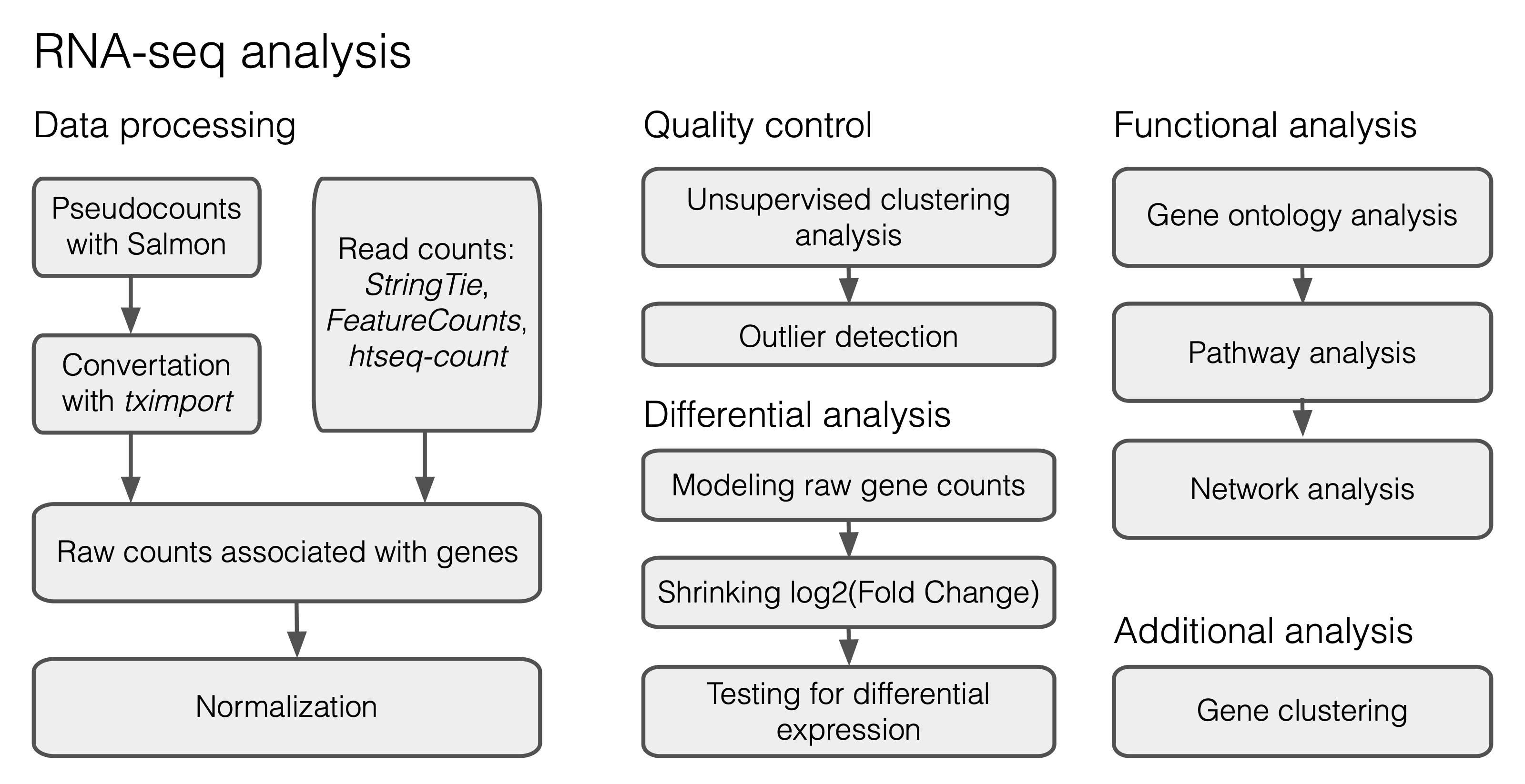
Fig. 2.1 A typical workflow for DE analysis.#
2.1. Preparing the data#
We will start with uploading expression data table together with meta file containing brief sample description (age, ethnicity). While original study include both male and females profiles, we selected only the male ones for the simplicity of the further analysis. Processed files (data_fibroblasts.csv and meta_fibroblasts.csv) are available here: http://arcuda.skoltech.ru/~d.smirnov/ComputationalAgingCourse/
import numpy as np
import pandas as pd
import sys
from collections import Counter

path_data = "data/data_fibroblasts.csv" # change this with your actual path to data file
raw_counts = pd.read_csv(path_data, index_col=0)
Check the number of gene features and number of samples available in the dataset:
print("Number of genes:", raw_counts.shape[0])
print("Number of samples:", raw_counts.shape[1])
Number of genes: 29744
Number of samples: 99
This table includes expression profiles of 99 samples with 29744 genes detected. However, some of this genes can have zero expression values across samples. We will filter them out:
raw_counts = raw_counts.loc[~(raw_counts==0).all(axis=1)]
raw_counts.shape
(24033, 99)
Then we will load meta file with sample descriptions:
path_meta = "data/meta_fibroblasts.csv" # change this with your actual path to meta file
meta = pd.read_csv(path_meta, index_col=0)
meta.head(10)
| Age | Ethnicity | |
|---|---|---|
| SRX4022456 | 1 | Asian |
| SRX4022457 | 12 | Caucasian |
| SRX4022459 | 25 | Caucasian |
| SRX4022461 | 26 | Caucasian |
| SRX4022463 | 28 | Caucasian |
| SRX4022464 | 29 | Caucasian |
| SRX4022465 | 29 | Caucasian |
| SRX4022466 | 30 | Caucasian |
| SRX4022468 | 30 | Caucasian |
| SRX4022469 | 30 | Caucasian |
Let’s check age range of our samples using the information from the first column of the meta
print("Minimal age:", min(meta.Age.values))
print("Maximal age:", max(meta.Age.values))
Minimal age: 1
Maximal age: 96
To perform further analysis we will divide samples into age groups with a step = 10 years.
df = pd.DataFrame(pd.cut(meta["Age"], np.arange(0, max(meta.Age.values)+10, 10), right = False, ordered = True))
df.columns = ['AgeBins']
df['AgeBins'] = df['AgeBins'].astype(str)
meta = pd.concat([meta, df], axis=1)
meta = meta.replace(np.unique(meta['AgeBins'].values), np.arange(10))
meta['AgeRanges'] = df['AgeBins'].values.astype(str)
meta.head()
| Age | Ethnicity | AgeBins | AgeRanges | |
|---|---|---|---|---|
| SRX4022456 | 1 | Asian | 0 | [0, 10) |
| SRX4022457 | 12 | Caucasian | 1 | [10, 20) |
| SRX4022459 | 25 | Caucasian | 2 | [20, 30) |
| SRX4022461 | 26 | Caucasian | 2 | [20, 30) |
| SRX4022463 | 28 | Caucasian | 2 | [20, 30) |
2.2. Setting up rpy2 functions#
from rpy2 import robjects
from rpy2.robjects.packages import importr
from rpy2.robjects import pandas2ri, Formula
import rpy2.robjects.numpy2ri
pandas2ri.activate()
robjects.numpy2ri.activate()
from rpy2.robjects.conversion import localconverter
from rpy2.rinterface_lib.embedded import RRuntimeError
deseq = importr('DESeq2')
sumexp = importr('SummarizedExperiment')
degreport = importr('DEGreport')
to_dataframe = robjects.r("function(x) data.frame(x)")
get_clusters = robjects.r("function(x) x[['df']]")
get_cluster_data = robjects.r("function(x) x[['normalized']]")
to_factors = robjects.r("function(x) data.frame(lapply(x,factor))")
class DESeq2():
    def __init__(self, counts, meta, design):
        self.raw_counts = robjects.conversion.py2rpy(counts.round().astype(int))
        self.meta_chr = robjects.conversion.py2rpy(meta)
        self.meta = to_factors(robjects.conversion.py2rpy(meta))
        self.design = design

    def create_deseq_object(self):
        self.dds = deseq.DESeqDataSetFromMatrix(countData=self.raw_counts, colData=self.meta, design=self.design)

    def normalization(self):
        self.dds = deseq.estimateSizeFactors_DESeqDataSet(self.dds)
        norm_counts = to_dataframe(deseq.counts_DESeqDataSet(self.dds, normalized=True))
        norm_counts = robjects.conversion.rpy2py(norm_counts)
        norm_counts.index = robjects.conversion.rpy2py(self.raw_counts).index
        norm_counts.columns = robjects.conversion.rpy2py(self.raw_counts).columns
        return norm_counts

    def transformation(self, method = "vst"):
        if method == "vst":
            mat = deseq.varianceStabilizingTransformation(self.dds, blind = True)
        elif method == "rlog":
            mat = deseq.rlog(self.dds, blind = True)

        mat = to_dataframe(sumexp.assay(mat))
        mat = robjects.conversion.rpy2py(mat)
        mat.index = robjects.conversion.rpy2py(self.raw_counts).index
        mat.columns = robjects.conversion.rpy2py(self.raw_counts).columns
        return mat

    def LRT_testing(self):
        try:
            dds_lrt = deseq.DESeq(self.dds, test="LRT", reduced = Formula("~1"))
            res_LRT = to_dataframe(deseq.results(dds_lrt))
            res_LRT = robjects.conversion.rpy2py(res_LRT)
        except rpy2.rinterface_lib.embedded.RRuntimeError:
            sys.exit()
        return res_LRT

    def clustering(self, cluster_mat):
        cluster_mat = robjects.conversion.py2rpy(cluster_mat)
        dp = degreport.degPatterns(cluster_mat, metadata = self.meta_chr, time = "AgeBins")
        cluster_content = robjects.conversion.rpy2py(get_clusters(dp))
        cluster_data = robjects.conversion.rpy2py(get_cluster_data(dp))
        return cluster_content, cluster_data
2.3. Normalization#
Specify a design formula for statistical testing with DESeq2 (it is important to put the factor of interest in the end of the formula!):
design = Formula("~AgeBins")
d = DESeq2(raw_counts, meta, design)
Initialize DESeq2 object with our data:
d.create_deseq_object()
Perform DESeq2 normalization:
ncounts = d.normalization()
Then transform data using variance stabilizing transformation (VST) to get rid of heteroskedasticity:
vst_mat = d.transformation(method = "vst")
2.4. Quality control#
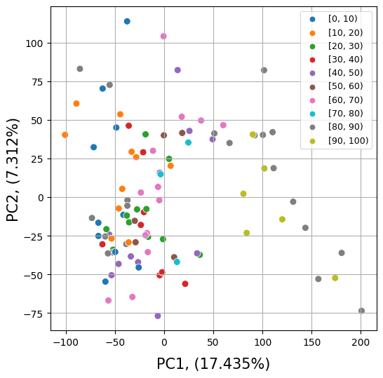
Before differential analysis we will explore a similarityof the samples in the age groups
2.4.1. Principal Component Analysis#
import matplotlib.pyplot as plt
import seaborn as sns
from sklearn.decomposition import PCA
from sklearn.preprocessing import StandardScaler
x = np.transpose(vst_mat.values)
x = StandardScaler().fit_transform(x)
pca = PCA(n_components=2)
principalComponents = pca.fit_transform(x)
principalDf = pd.DataFrame(data = principalComponents, columns = ['PC1', 'PC2'])
pcdf = pd.concat([principalDf.set_index(meta.index), meta], axis = 1)
fig, ax = plt.subplots(figsize=(6, 6))
sns.set_context("paper", font_scale=1.5)
sns.scatterplot(data=pcdf, x="PC1", y="PC2", hue="AgeRanges", s = 50)
plt.legend(loc="upper right", fontsize=5)

var_pc1 = (pca.explained_variance_ratio_[0]*100).round(3)
var_pc2 = (pca.explained_variance_ratio_[1]*100).round(3)
plt.xlabel('PC1, ('+ var_pc1.astype(str) + "%)", fontsize = 15, labelpad = 10)
plt.ylabel('PC2, ('+ var_pc2.astype(str) + "%)", fontsize = 15, labelpad = 2)

handles, labels = plt.gca().get_legend_handles_labels()

order = [0,1,2,3,4,5,6,9,7,8]
plt.legend([handles[idx] for idx in order],[labels[idx] for idx in order], fontsize=9)

ax.grid()
Exercise 1
Perform PCA on the top 500 most variable genes in the dataset (1 point).
2.5. Statistical testing#
Run Likelihood Ratio Test (LRT) available in DESeq2 package:
%%capture
res = d.LRT_testing()
Sort genes by the adjusted p-value:
res = res.sort_values(by=['padj'])
Retrieve all the genes satisfying p-value cut-off criteria \(P<0.05\):
sig = res[res['padj'] < 0.05]
Check the number of significant genes:
print("Number of DE genes:", sig.shape[0])
Number of DE genes: 8449
Exercise 2
Define the number of up- and down-regulated genes in the analysis (0.5 points). Investigate the top 10 DE genes from up and down lists. Do they have any established connection with aging? If yes, support your claim with some references and short description of their functions. (1.5 points).
2.6. Gene clustering#
To perform gene clustering we will select only a subset of significant genes, let’s say 1800 the most significant features
ngenes = 1800
cluster_mat = vst_mat.loc[sig.head(ngenes).index]
Perform gene clustering by executing degPatterns functions from DEGreport R package:
%%capture
content, clust_data = d.clustering(cluster_mat)
The function above returned 15 clusters consisting of more than 16 genes that are simialar in thir expression patterns.
Counter(content.cluster.values)
Counter({1: 248,
         2: 415,
         3: 110,
         4: 471,
         5: 36,
         6: 186,
         7: 56,
         8: 20,
         9: 35,
         10: 18,
         11: 16,
         12: 37,
         14: 42,
         17: 16,
         20: 40})
We can use a content from clust_data dataframe to explore obtained expression patterns and plot them with seaborn library
g = sns.catplot(data=clust_data,
                x='AgeRanges',
                y='value',
                col='cluster',
                kind='box',
                col_wrap=5,
                order= np.unique(clust_data.AgeRanges.values))
g.set_axis_labels("", "Z-score of gene abundance")
g.tick_params(axis='x', rotation=45)
axes = g.axes.flatten()
gene_number = Counter(content.cluster.values)
cluster_ids = list(gene_number.keys())
for i in range(len(axes)):
    axes[i].set_title("Cluster " + str(cluster_ids[i]) + ", [" + str(gene_number[cluster_ids[i]]) + " genes]")
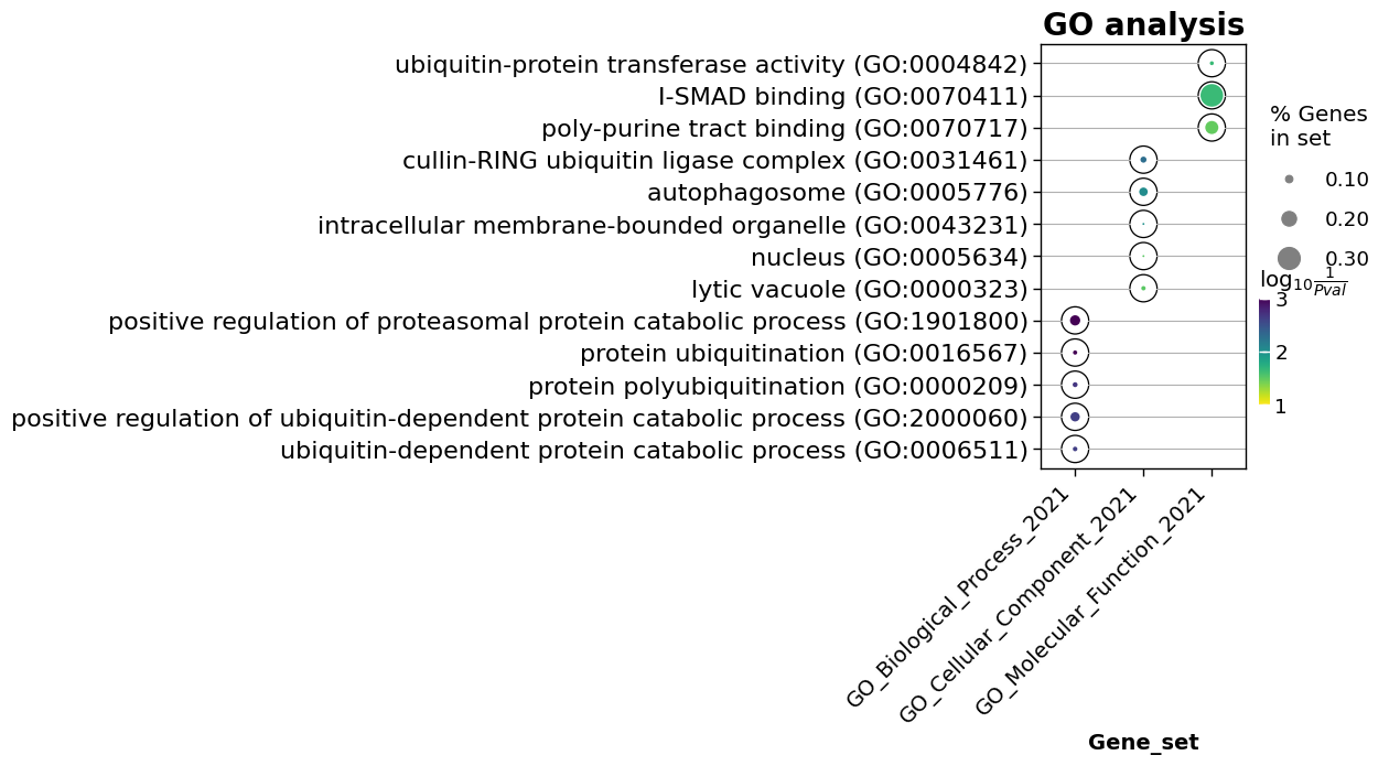
2.7. GO analysis#
import gseapy
from gseapy import barplot, dotplot
Select a cluster for the GO analysis:
cluster_id = 2
enr = gseapy.enrichr(gene_list = list(content[content['cluster'] == cluster_id].genes.values),
                     background = res.index.values,
                     gene_sets=['GO_Biological_Process_2021',
                                'GO_Cellular_Component_2021',
                                'GO_Molecular_Function_2021'],
                     organism='human',
                     outdir=None)
For the simplicity we will drop non informative columns and keep the terms posessing ‘Adjusted P-value’ < 0.05
enr_res = enr.results.iloc[:,[0,1,2,4,9]]
enr_res = enr_res[enr_res['Adjusted P-value'] < 0.05]
To visualize top 5 enrichment terms from each set (Biological Process, Cellular_Component, Molecular Function) we can apply dotplot function from gseapy:
dotplot(enr_res,
              column="Adjusted P-value",
              x='Gene_set',
              size=10,
              top_term=5,
              figsize=(3,5),
              title = "GO analysis",
              xticklabels_rot=45,
              show_ring=True,
              marker='o',
             )
<AxesSubplot:title={'center':'GO analysis'}, xlabel='Gene_set'>
Exercise 2
Perform GO analysis on genes from clusters 1, 3, 4 and prepare figures showing the top 5 enriched terms (if possible) (1 point).
Exercise 3
Perform enrichment analysis on genes from cluster 1, 3, 4 using aging related databases: ‘Aging_Perturbations_from_GEO_down’, ‘Aging_Perturbations_from_GEO_up’ and ‘GTEx_Aging_Signatures_2021’ (1 point).
2.8. Learn more#
Detailed manual on differential expression analysis with DESeq2 in R
RNA-seq analysis with Python
Omics Data Analysis course at Skoltech (MA060061)
2.9. Credits#
This notebook was prepared by Dmitrii Smirnov.
2.10. References#
[1] Fleischer, J.G., Schulte, R., Tsai, H.H. et al. Predicting age from the transcriptome of human dermal fibroblasts. Genome Biol 19, 221 (2018). https://doi.org/10.1186/s13059-018-1599-6”